量化交易学习(十五)Qlib人工智能量化框架快速入门(2)
上一篇文章跟着一篇研报过了一遍安装流程,以及一些数据获取相关的命令。今天在跑研报提供的例子的时候发现有些代码已经跑不通了,估计是qlib有些api已经改了,在qlib源码中的examples找到了官方的入门例子。
workflow_by_code.ipynb 与 workflow_by_code.py 是用qlib跑回测的完整流程代码。在 tutorial 目录中的 detailed_workflow.ipynb 是详细工作流程的代码。
接下来照着 workflow_by_code.ipynb 把整个流程跑一遍。
导入 qlib 库:
1 | import os |
初始化数据
1 | # use default data |
设置股票池为沪深300中的股票,基准为沪深300指数:
1 | market = "csi300" |
训练模型:
模型采用GBDT,训练特征采用Alpha158
1 | ################################### |
预测、回测以及数据分析:
回测的策略使用TopkDropout。
TopkDropout 策略如下:
- TopK: 持有的股票数
- Drop: 每天卖出的股票数
在每个交易日,卖掉预测分最低的Drop个股票,同时买入同等数量的评分最高的其他股票。这样就保证了换手率。
1 | ################################### |
分析图表:
1 | from qlib.contrib.report import analysis_model, analysis_position |
分析头寸
报告:
1 | analysis_position.report_graph(report_normal_df) |
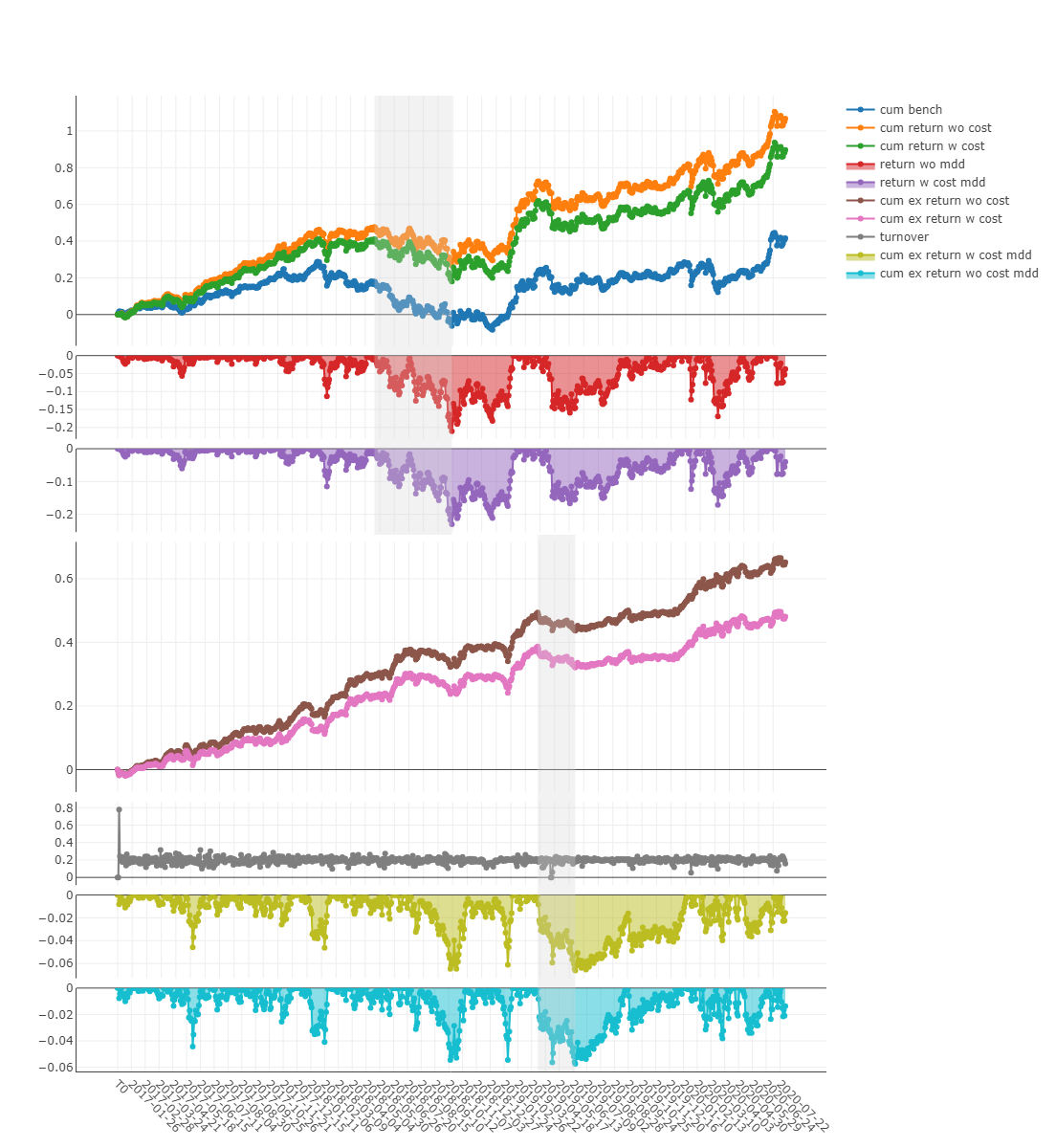
图片上,x轴为交易日,y轴上不同的曲线含义不同:
- cum bench 基准累积收益率
- cum return wo cost 不含交易费的投资组合累积收益率
- cum return w cost 包含交易费的投资组合累积收益率
- return wo mdd 不含交易费的累积收益最大回撤
- return w cost mdd 包含交易费的累积收益最大回撤
- cum ex return wo cost 不含交易成本基准下,投资组合的总超额收益
- cum ex return w cost 计入交易成本基准下,投资组合的总超额收益
- turnover 换手率
- cum ex return wo cost mdd 不计交易成本,投资组合超额收益的最大跌幅
- cum ex return w cost mdd 计入交易成本,投资组合超额收益的最大跌幅
- 上半部分的阴影表示 不含交易成本的累积收益所对应的最大亏损
- 下半部分的阴影表示 不含交易成本的超额收益对应的最大回撤
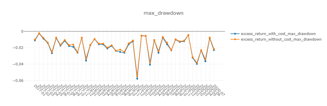
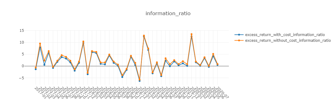
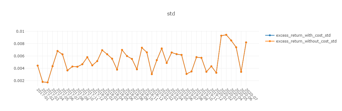
风险分析:
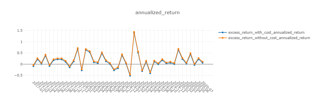
1 | analysis_position.risk_analysis_graph(analysis_df, report_normal_df) |
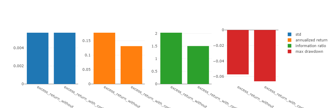
图表说明:
- std 标准差
- annualized_return 年化收益率
- information_ratio 信息比率(Information Ratio – IR).
- max_drawdown 最大回撤
- excess_return_without_cost 不计交易成本累计超额收益 (CAR)
- excess_return_with_cost 含交易成本的累计超额收益 (CAR)
下面图表中,x轴为按月聚合的交易日。
分析模型
1 | label_df = dataset.prepare("test", col_set="label") |
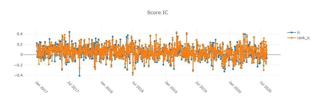
图中x轴为交易日,y轴的含义如下:
- ic 标签和预测分数之间的皮尔逊相关系数,在例子被公式化为 Ref($close, -2)/Ref($close, -1)-1
- rank_ic 标签和预测分数之间的斯皮尔曼等级相关系数
模型性能
1 | analysis_model.model_performance_graph(pred_label) |
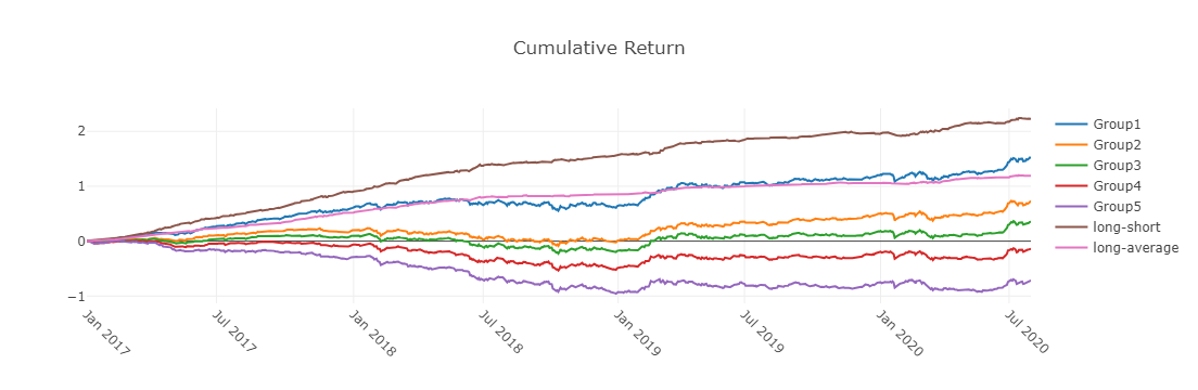
累积回报图
- Group1:The Cumulative Return series of stocks group with (ranking ratio of label <= 20%)
- Group2:The Cumulative Return series of stocks group with (20% < ranking ratio of label <= 40%)
- Group3:The Cumulative Return series of stocks group with (40% < ranking ratio of label <= 60%)
- Group4:The Cumulative Return series of stocks group with (60% < ranking ratio of label <= 80%)
- Group5:The Cumulative Return series of stocks group with (80% < ranking ratio of label)
- long-short:The Difference series between Cumulative Return of Group1 and of Group5
- long-averageThe Difference series between Cumulative Return of Group1 and average Cumulative Return for all stocks.
The ranking ratio can be formulated as follows.
𝑟𝑎𝑛𝑘𝑖𝑛𝑔 𝑟𝑎𝑡𝑖𝑜=(𝐴𝑠𝑐𝑒𝑛𝑑𝑖𝑛𝑔 𝑅𝑎𝑛𝑘𝑖𝑛𝑔 𝑜𝑓 𝑙𝑎𝑏𝑒𝑙) / (𝑁𝑢𝑚𝑏𝑒𝑟 𝑜𝑓 𝑆𝑡𝑜𝑐𝑘𝑠 𝑖𝑛 𝑡ℎ𝑒 𝑃𝑜𝑟𝑡𝑓𝑜𝑙𝑖𝑜)
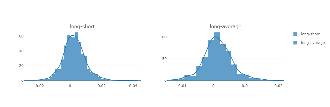
long-short/long-average
The distribution of long-short/long-average returns on each trading day
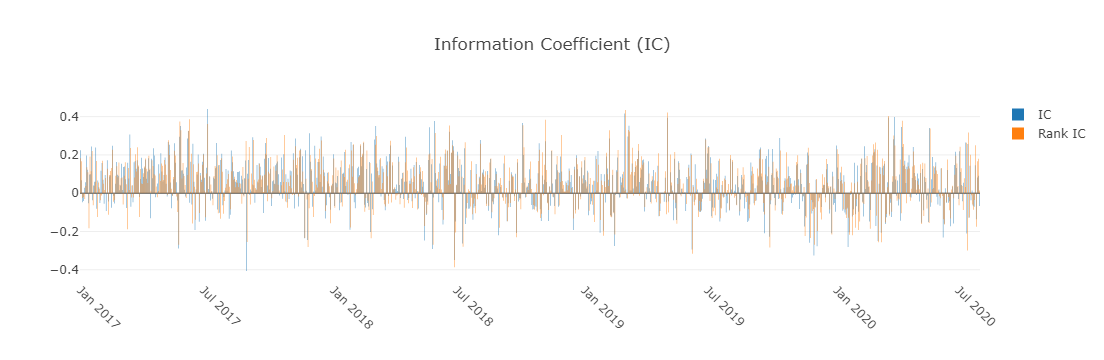
- Information Coefficient
- The Pearson correlation coefficient series between labels and prediction scores of stocks in portfolio.
- The graphics reports can be used to evaluate the prediction scores.
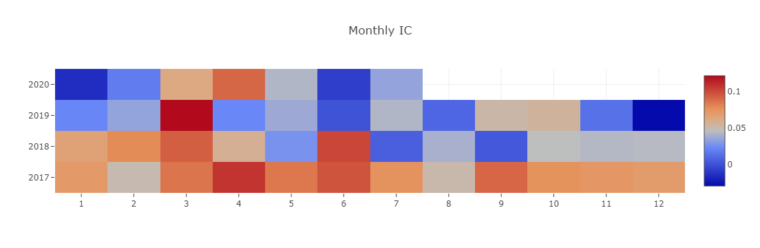
- Monthly IC
- Monthly average of the Information Coefficient

- ICThe distribution of the Information Coefficient on each trading day.
- IC Normal Dist. Q-QThe Quantile-Quantile Plot is used for the normal distribution of Information Coefficient on each trading day.
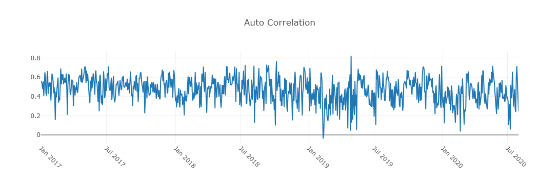
- Auto Correlation
- The Pearson correlation coefficient series between the latest prediction scores and the prediction scores lag days ago of stocks in portfolio on each trading day.
- The graphics reports can be used to estimate the turnover rate.